Fundamentals of Feedback Control using Microcontroller [Extra Edition]

The inverted pendulum is a typical teaching tool of modern control theory. The information that is generally available is either too academic or too much trial-and-error, and there is not much that has been systematically verified so that even beginners can understand it.
Table of contents
Application of Modern Control Theory

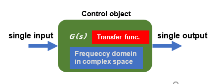
So far, I have verified feedback control based on transfer functions. This is the so-called classical control approach. In principle, it is possible to control a system with one-input and one-output, which is suitable for most of the familiar feedback control such as temperature control and motion control of a single motor.
In contrast, a typical, slightly more complex system is the control of an inverted pendulum. Taking a cart-type inverted pendulum as an example, an inverted pendulum is inherently unstable, but to maintain a stable inverted state, the position of the cart is constantly balanced with the pendulum's center of gravity by fine-tuning the position of the cart.
The purpose of the control is to make the inverted angle of the pendulum perpendicular to the cart, but in order to control the indirect position of the cart at the same time, the system is a so-called one-input, multiple-output system that takes pushing force and other inputs.
It is not impossible to control the cart position and pendulum angle simultaneously by setting the gains appropriately with classical PID control, etc., but it is not feasible because such ad hoc adjustment is difficult and makes the control system more complicated.
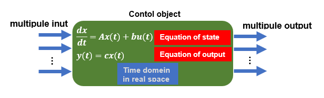
Modern control theory is suitable for simultaneously stabilizing multiple variables such as cart position and pendulum angle. In modern control theory, multiple variables handled inside a system are called state variables, and this theory is used to stabilize them simultaneously.
If you read a modern control theory manual, you will almost certainly lose heart if you study it on your own because it is so mathematical, but the essence of the theory is not difficult if you know what you are looking for.
Even without understanding the mathematical formulas, it is now easy to understand modern control theory, which is often thought to be difficult to understand, because free and convenient tools are now available to actually try out various things.
Therefore, I would like to confirm the amazing aspects of this theory through a typical application of modern control theory, the inverted pendulum.
What is an inverted pendulum?
Inverted pendulums can be broadly classified into two types: the cart type, in which the pendulum is mounted on a cart with a fulcrum, and the wheel type, in which the fulcrum of the pendulum is on two wheel axles.
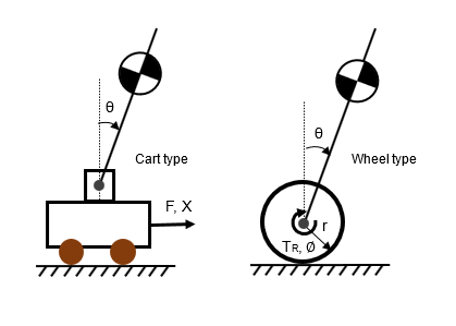
In the cart-type inverted pendulum, the position X of the cart is adjusted by the applied thrust F to set the pendulum angle θ close to zero, and the equation of motion is relatively simple and there is not much interference between the bogie and the pendulum, so it is said to be easy to control.
In contrast, the wheeled inverted pendulum uses torque TR to adjust the rotation angle Φ of the wheel to bring the pendulum angle θ close to zero, but the equations of motion are a little more complicated because torque TR affects the rotation of the pendulum as well as the translation of the wheel, and they interfere with each other.
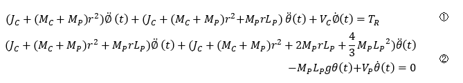
Wheeled inverted pendulum equation of motion
In this part, I will apply modern control theory to the inverted pendulum and verify its usefulness through simulation. Later, I would like to verify it using an actual LEGO machine, so I will deal with a wheel-type inverted pendulum accordingly.
The equations of motion for a wheeled inverted pendulum are quite complex and difficult to calculate.
The following model is used here, omitting the calculation process.
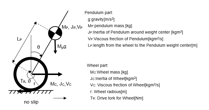
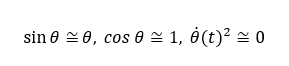
(1) is the equation of motion for a wheel and (2) is the equation of motion for a pendulum. The following approximations and linearizations are used to derive them.
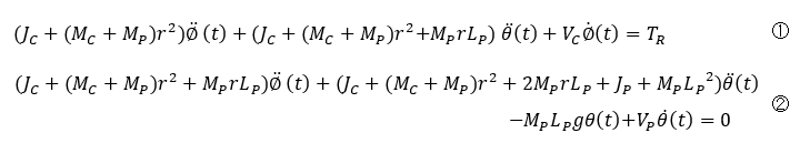
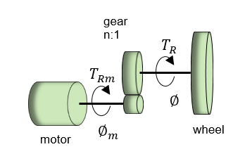
The input is voltage or current to the motor, and the wheels are connected to the motor shaft by gears and other transmission mechanisms. The mass and moment of the wheel and pendulum affect each other, resulting in a complicated equation.
Approximate model method
The first step in control is to have a mathematical model to serve as a base, so I have been working hard to derive the equations of motion.
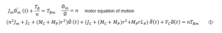
Usually, in academic papers, it seems that torque is calculated based on the derived equation of motion (1)' and converted to the equivalent voltage or current as input, but in practice, it is difficult to obtain motor shaft inertia, viscous friction, etc. Even if all the parameters could be obtained, the parameters would still fluctuate, and I think the torque calculation method is not practical from a practical standpoint.
In other words, what we want to control is the pendulum angle and the position of the wheel or bogie, but no matter how much torque or thrust force is obtained from complex mathematical formulas, they are indirect and not very reliable.
Therefore, I explained the approximate model in "Fundamentals of Feedback Control using Microcontroller[Advanced]" and here, too, I use a transfer function that approximates the voltage or current input u to the output wheel speed with a 1st-order lag.
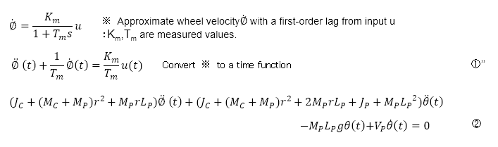
The equation of wheel motion (1)" is now a very simple and practical model. However, the interference terms due to the pendulum (two items in equations (1) and (1)') are ignored. The equation of motion of the pendulum (2) is still complicated, but since we are still in the simulation stage, we assume that the parameters are known.
The pendulum part is also approximated in the implementation model, but the most important parameters of the pendulum are the period and damping characteristics, so these parameters alone must be identified and obtained.
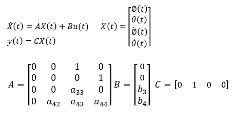
The equation of motion (1)''(2) is transformed to form the equation of state (3)(4). This is the equation of state for a wheeled inverted pendulum that approximates the wheel model.
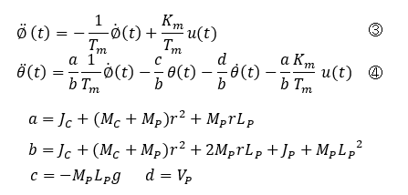
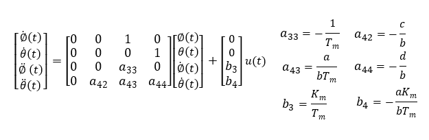
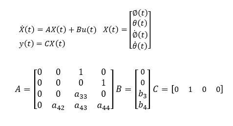
I will rewrite it in the following format for consideration in modern control theory. In this way, the analysis can finally begin in the familiar format of modern control.
The problem with this method is that it ignores the effect of the pendulum in making the approximation. In other words, when the input u is voltage or current, the wheel speed is actually interfered with to some extent by the pendulum's motion as a disturbance load. The wheel speed input method described next solves this problem.
Wheel speed input method
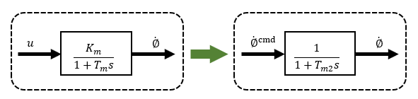
The previous inverted pendulum using the wheel approximation model was practical enough, but I will go one step further and consider the case where the input is not voltage or current as before, but wheel speed.
Although the use of motor voltage and current as inputs simplified the system, it did not solve the problem of pendulum effects (interference) on the wheels. Therefore, the speed control system is now made more robust by using the wheel speed as the input, so that the wheel is not affected by the pendulum.
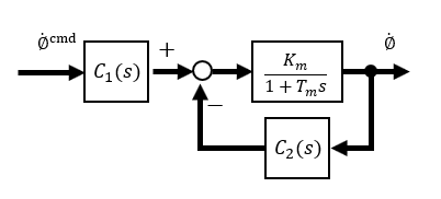
As explained in my previous article on robust control of DC motors, 2-degree of freedom control is a completely robust control, but this time I will verify wheel speed control using a simple High-gain feedback method.
The state equation for the case where the output has a 1st-order lag relative to the wheel speed input in wheel speed control is shown in (5) and (6). The wheel equation is characterized by the fact that the only parameter is the time constant Tm2, which can be set arbitrarily.
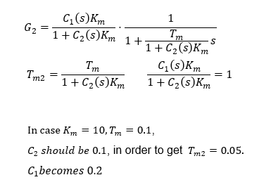
Since this is a High-gain feedback system, the larger the feedback gain C2, the more robust it is. At the same time, however, it also affects the time constant Tm2, which should be set at a feasible level so that it does not become too small.
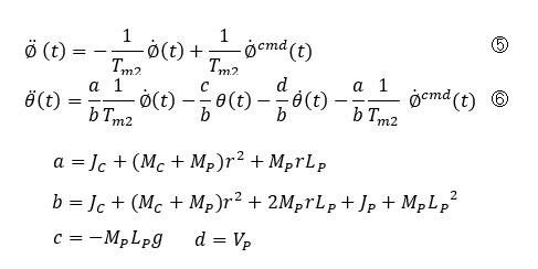
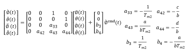
It is an equation of state in modern control theory form. Formally, it is similar to the approximate model method with voltage and current as inputs, but the content is completely different.
Since the wheel speed control system has improved disturbance suppression, the wheel speed follows the command input without being affected by the pendulum. The difference is that the pendulum is stabilized not by wheel torque as in the past, but by wheel speed.
Stabilization by state feedback
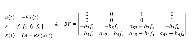
In modern control theory, it is possible to stabilize an unstable system by applying state feedback, in which each state variable handled is multiplied by a gain and returned to the input.
This way, even if the original matrix A of the entire system is unstable (eigenvalues of matrix A are unstable), the matrix A-BF with state feedback can be stabilized by setting the gain appropriately.
The eigenvalues of the system matrix are equivalent to solutions of specific equations in classical control, and the stability of all eigenvalues means that the state variables converge to zero over time.
Modern control theory sometimes requires evaluation of controllability or observability, but here I assume that both are possible.
Pole placement method
Just as in classical control, the poles are arranged so that all solutions of the characteristic polynomial of the transfer equation are stable, in modern control theory, the method of calculating the state feedback gain by setting the poles arbitrarily and stabilizing all eigenvalues of the system matrix is called the pole placement method.
We know that a stable pole has a negative real number part, but we do not know quantitatively how to determine the value setting to achieve practical operation on an actual device. To some extent, it is a matter of trial and error. The method used for qualitative and quantitative evaluation is the optimal regulator described below.
Optimal regulator (LQ optimal control)
In extreme cases, even if you use the pole placement method, you will not know what the correct answer is, so you will want an indicator for evaluation. The optimal regulator is a powerful tool in such cases.
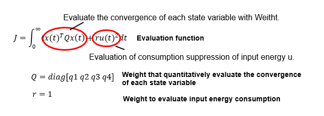
Leaving aside the mathematics of the optimal regulator, what the equation means is that the convergence of each state variable and the evaluation index of the suppression of consumption of input energy u are represented by J, and the objective is to obtain a feedback gain that is pole-positioned so that J is minimized.
The weight Q for each state variable can be set to a large or small value depending on which variable convergence is important. If convergence is important, a large number of operations are required, so the value cannot be set too large blindly if it is not feasible. The energy consumption weight r is usually set to 1.
The final determination of weights is where adjustments are made using simulation software or actual equipment. Compared to the pole placement method, this method is more realistic in that there is an evaluation index to guide the adjustment.
The simulation software Scilab makes it easy to design by allowing you to specify arbitrary poles for the pole placement method and arbitrary weights for the optimal regulator, and it will calculate the feedback gains for each state variable accordingly.
Aside from the difficult mathematical evaluation, it is now possible to use modern control theory with some ease.
Modern control theory, like classical control theory, is not difficult once you get the hang of it. Aside from its mathematical significance, it is a shortcut to understanding control theory to make use of convenient simulation applications that are now available free of charge.
Simulation
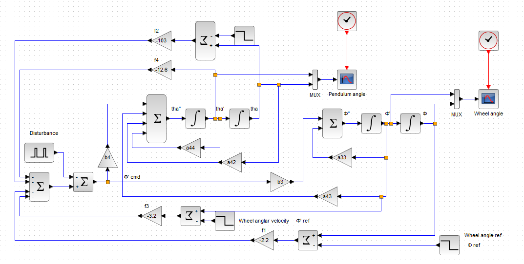
The optimal regulator set the weights to Q=diag[5 5 1 1] and r=1, and the gain obtained from the evaluation was F=[-2.2 -103 -3.2 -12.6], so the designed block diagram is shown below.
Simulation Parameters :
MC:0.06kg / MP=1.2kg / LP=0.065m / r:0.04m / Tm:0.1s / Tm2:0.05s / Km:10 / vp:0.03kgm2/s / JC:MCr2/2 /JP:1/3MPLP2:
Normally, the state variable X converges to zero over time, but here is the response when the wheel position (angle) is set to 5 as the target value Φref (Φ'=Φ-Φref). The state variable wheel position Φ with a target value other than zero corresponds to Φ'.
It is characterized by the fact that the state-feedback input u(t) is a wheel speed command as follows.
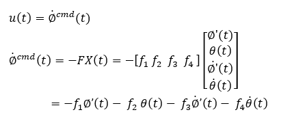
In the actual machine, this means that if the machine can be operated in such a state, it can be stably inverted while simultaneously changing the position of the wheels.
Incidentally, the eigenvalues of system matrix A before applying state feedback are [-8.2 6.2 0 -20.0], which are unstable because they contain positive values, while the eigenvalues of system matrix A-BF after applying state feedback are [-29.2 -7.5 -6.5 -1.6], all stable values.
This means that the system matrix A, i.e., the wheeled pendulum before applying state feedback, remains unstable without any input, and the system matrix A-BF, to which the input with state feedback is applied, stabilizes both the pendulum inversion and the wheel position at the same time.
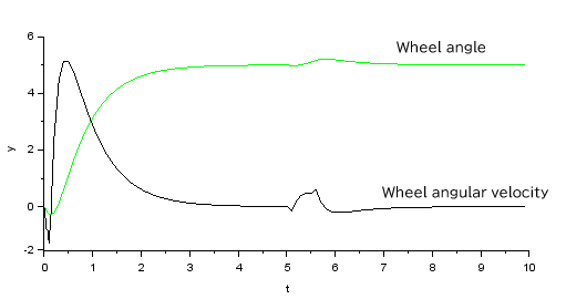
Wheel position and velocity response:
Immediately after starting with the pendulum angle zero (vertical), the wheel position is instantly retracted to make the pendulum bend forward, but it appears to converge to the target value of 5.
The input is slightly disturbed by the pulsed disturbance at the 5s, but all state variables are stable and convergent.
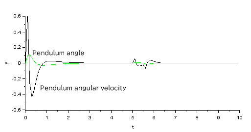
Pendulum angle and angular velocity response:
The pendulum angle is stable, although there is a slight undershoot, as it attempts to converge to zero immediately after the pendulum is bent forward at startup. It also converges when a disturbance is applied.
Since the commonly available inverted pendulum control is neither new nor interesting, I have tried to organize it from a hybrid perspective with classical control, incorporating a more practical robust control of the motor, so to speak. Next, I would like to explore the simplest and most stable control by using an actual machine to verify various aspects.
The inverted pendulum was inevitably difficult to evaluate and design using only the transfer function in a classical control approach, so I tried to incorporate modern control theory. Modern control theory is suited to the control of advanced and complex systems such as Aircraft, Satellite, and Drone attitude control, and although I am not sure if it is generally practical, it may be useful in some cases if you understand it.

