Fundamentals of Feedback Control using Microcontroller [Preparation]
I have summarized in my own way the outline of control theory, which will expand the world of design and development if it is mastered in order to realize motion control using embedded MCUs. This is not a sequence control in which commands are executed in order as in programming, but a feedback control in which the output of the controlled object is returned to the input side for comparison and correction.
Feedback control is generally referred to as Control engineering, and what is written in commercial books and textbooks is rather mathematical than physical, too abstract for beginners to understand on their own. Therefore, as much as possible, I have tried to summarize the points with an awareness of what mathematical things mean in physical terms.
This site specifically covers DC motors and their surrounding electrical circuits, etc., so that feedback control can be handled in motion control, which will be introduced in the future, and I would like you to get an overview. Once you have a certain level of understanding, I believe that you will be able to further deepen your understanding of the essence of the subject by referring to the various expressions and explanations provided by various people on the Internet to expand your knowledge of the content from a different angle.
In this preparation section, I will explain how to model the control target object using the circuit equation and the mechanical equation of a DC motor. The analysis section explains the key points when providing appropriate feedback information to the modeled control object. In the application section, I introduce the techniques actually used in the field, such as PID control and speed control of DC motors.
Table of contents
- 1 What is feedback control...and how does it differ from general Sequence control?
- 2 Classification of Control Theory
- 3 Preparation for understanding control theory
- 3.1 About Complex Numbers
- 3.2 Why complex number j is used in electric circuits
- 3.3 Why design in complex number space in the frequency domain in control theory?
- 3.4 Modeling of the control object
- 3.5 Laplace transform: (transformation from time space to complex number space)
- 3.6 Block Diagram Representation by Transfer Function
What is feedback control...and how does it differ from general Sequence control?

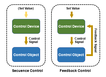
Generally speaking, automatic control is broadly classified into Sequence control and Feedback control. Sequence control is a process that functions according to the conditions set in a combined or programmed process using relay circuits, etc. It is also called open-loop control or open-loop control.
A PLC (Programmable Logic Controller) that controls industrial machinery is a typical sequence control. Familiar examples include traffic signals, which function by means of programs that use timers and conditional branching in sequence control.
In contrast, Feedback control refers to automatic control in which the output of the controlled object is fed back (returned to the input side) to make corrective actions to bring the measured value by a sensor, etc. closer to a set target value. It is also called closed-loop control. A familiar example is the temperature setting of an air conditioner. Driving a car can also be considered feedback control, since the brain makes judgments based on visual and other information and controls the car.
Instead of a person controlling the autocruise function of an automobile by sensing the speed from the meter or engine noise, an on-board sensor detects the speed and provides feedback to the engine to adjust the power output to the engine.
Feedback control has advantages that sequence control does not have, but because it uses feedback information, it can become very unstable if there is a defect in the way it is corrected. In other words, if the signals and information to be corrected are always close to the target values, the system is stable, but if they move away from the target values due to various factors (disturbances), the system may become unstable in a so-called vicious circle due to the closed-loop nature of the system.
Hunting, often heard in the field, is a phenomenon in which a mechanical feedback system that involves movement becomes oscillatory due to poor adjustment, while howling is a phenomenon in which a microphone picks up sounds other than voice from the output speaker, creating a closed loop and causing an unstable state. The term "unstable" refers to a state of instability caused by an irresistible amplification of the signal.
For this reason, the first important item for designing feedback control is stability, and trackability to the target value. In addition, strong disturbance suppression (robustness) against various fluctuation factors, external disturbances, noise, etc. may also be required.
Feedback control design has long been a well-established theory and an academic subject, but even if the general public were to look at a book or textbook on "Control engineering" without prior knowledge, it would be difficult for them to understand the almost mathematically abstract content, and frankly, they might not find it interesting at all. The following is an example of a case in point.
Recently, with the spread of the Internet, it has become possible to find explanations of this difficult and abstract subject from various angles using concrete examples, so that even self-study is possible if one is serious about it, but it is still difficult to become familiar with mathematical formulas.
Therefore, in this site, I intend to explain specific and essential aspects of motor control in particular without relying on mathematics as much as possible. Even so, there are still certain mathematical and physical aspects that are essential and cannot be avoided, so please do your best to understand them.
Classification of Control Theory
Control theory is academically classified into Classical control and Modern control.
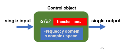
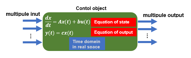
Classical control is simply put, a control theory that evaluates and analyzes in the frequency domain (complex number space) based on a transfer function model. On the other hand, Modern control theory is a control theory that evaluates and analyzes in the time domain (real number space) based on a state space model.
These are not to be taken as old or new classifications as the names imply, but rather different approaches to control, both of which have their advantages and disadvantages. Other derivatives include Robust control and Adaptive control, which are control methods that have evolved from classical and modern approaches.
This site covers what is called Classical control, which is analyzed in the frequency domain (complex number space). In addition to the fact that I have a background in electrical engineering, the idea of using transfer functions as a base is to construct a kind of special filter between inputs and outputs, and the fact that it can be designed physically, rather than mathematically, suits my nature.
The appearance is intuitive, as it can be constructed as a block diagram by a transfer function transformed into complex number space with complex number s as a variable. The point is complex numbers, but you just need to get used to complex numbers as a convenient tool rather than treating them as a mathematical concept. The great advantage of the classical control method based on transfer functions is that the modeling parameters can be done with a certain degree of accuracy, but not so strictly because of the filter concept.
Modern control theory is based on analysis in the time domain, which is rather mathematical and involves modeling the control object in terms of differential equations called Equations of state. Although it is difficult to solve differential equations, nowadays, this is not a problem because the computer can analyze the equations instead of human hard works. Compared to classical control, the modeling parameters require a certain degree of precision. Since the state variables used in the state equation are handled, the system can be analyzed as a multi-input, multi-output system.
To summarize the characteristics of the two, classical control theory is based on transfer functions in complex space in the frequency domain for design evaluations such as system stabilization, while modern control theory is based on equations of state, which are differential equations, for mathematical analysis and design in actual time space.
Classical control theory is easier to understand if the emphasis is on physical evaluation, while modern control theory is better suited for advanced analysis of internal parameters with an emphasis on calculation.
For example, in the case of a cart-type inverted pendulum, the angle of the pendulum and the position of the cart are used as state variables to control the angle of the output pendulum by operating the actuator's torque, etc. The relationship between input and output is complicated, and the characteristics cannot be easily predicted with a single transfer function.
In this example, there are many variables from input to output, and modern control theory is well suited for capturing their states. With appropriate state feedback, the system can be stabilized very easily. Classical control theory using transfer functions can also be used, but it seems to be a little too difficult.
Modern control theory has some advantages that classical control theory does not have, but it is more of a mathematical analysis, so if you are a beginner in control and good at mathematical interpretation, you can learn from modern control theory, but if you want to focus on physical interpretation, it would be better to start from classical control theory. I think it is a good idea. The key is not so difficult.
In my personal view, the best way to utilize the advantages of both modern and classical control theory is not to divide them in two, but to merge them according to the application. For example, modern control theory is utilized to optimally manage and control a large, complex system as a whole, while classical control theory is utilized to control the individual parts used within that system to ensure performance.
Preparation for understanding control theory
Classical control theory expresses control models in the real-time domain in terms of transfer functions in the frequency domain (complex number space) and then performs evaluation and analysis. The purpose of this course is to understand the concept of complex numbers and how to use a tool called Laplace transform to convert a control object into a transfer function model and then to create a block diagram.
Many control theory explanations often make extensive use of mathematical formulas, but this site focuses on the minimum necessary to realize motion control using DC motors, but it is still sufficient for practical use.
About Complex Numbers
Complex numbers are a great concept!!
In mathematics, an imaginary number is simply a number j that, when squared, becomes j2=-1 (in electrical and control engineering, j is used to distinguish it from the current i), however, when this concept of imaginary numbers is applied to physics as a tool, it can be turned into something very useful.
A complex number Z is a combination of the real part a and the imaginary part jb, Z=a+jb. In real number space, for example, current i(t) is a scalar quantity (magnitude itself) that only increases or decreases with parameter t (time), whereas in complex number space, it can be expressed as a vector quantity (having magnitude and phase) with Z=a+jb.
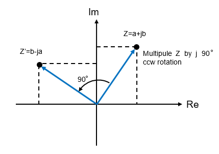
In other words, Z=a+jb means that the imaginary part b is on the imaginary axis counterclockwise by 90° relative to a on the real axis. Multiplying a complex number by an imaginary number j has the property that the vector of that complex number will be in a position rotated 90° counterclockwise around the origin.
Taking advantage of this property, electric circuits and equations of motion can be converted to complex number space, which is much easier to analyze and handle than when expressed in real number space (the world of differential equations). Incidentally, the concept of complex numbers is not used in physics up to high school, but first appears in college.
Complex numbers used in engineering should be thought of as a useful tool that makes use of their properties rather than as a mathematical essential.
Why complex number j is used in electric circuits
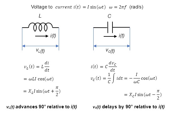
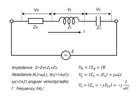
In electrical engineering, the complex number plane is used to analyze circuits. A DC circuit with only resistance R can be handled using only real numbers, which can be understood intuitively by anyone because Ohm's law holds true. On the other hand, in the case of an AC circuit combined with an inductor L and a capacitor C, the operation cannot be explained simply by Ohm's law of real numbers.
This is because the phase of the voltage across the coil L and capacitor C with respect to the AC current (sinusoidal) flowing through them is advanced in the coil and delayed in the capacitor C. Therefore, using the complex number plane, which can include not only the effective values of current and voltage but also phase information, makes it possible to handle the circuit as a vector and simplifies it.
This is a bit off topic, but let me verify physically, without using mathematical formulas, why the phase of the voltage shifts with respect to the current in a coil and a capacitor.
The phase shift of the inductor L and capacitor C can be expressed by the following equation. This formula is valid for time-varying circuits. We can see that for a sinusoidal alternating current flowing through a coil and a capacitor, the phase of the voltage on each end advances by 90° (π/2) for the coil and delays by 90° for the capacitor, respectively. I will represent this in complex number space.
In a DC circuit with only resistance R, the resistance is only real, whereas in an AC circuit combined with a coil L and a capacitor C, the impedance Z is called impedance Z. The impedance ZL is jXL due to the inductive reactance XL (=ωL) of the coil in addition to the resistance R, and the capacitive reactance XC (=1/ωC ) is -jXC, so when the resistor R, the coil, and the capacitor are connected in series, the overall impedance is
Z = R + j(XL-XC) = R + j(ωL-1/ωC) is a vector of complex numbers.
Multiplying the original vector of complex numbers by "j" means a phase advance of 90°, while multiplying by "-j" means a phase delay of 90°.
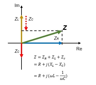
In a series circuit with a common current flow, the phase of the voltage VL across the coil is 90° ahead of the phase of the voltage VR across the resistor R , and 90° behind the phase of the voltage VC across the capacitor, based on the formula defining the impedance Z.
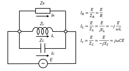
In a parallel circuit with a common voltage, the currents flowing in the resistor, inductor, and capacitor are delayed in phase by 90° in the inductor and advanced in phase by 90° in the capacitor.
When this complex vector is handled, it is very convenient to analyze the frequency characteristics between input and output, as well as the phase characteristics, with relative ease.
Why design in complex number space in the frequency domain in control theory?
In so-called classical control, which treats the transfer function between input and output as a transfer function, the input is the target set value and the output is the physical quantity to be controlled, and the entire system including the transfer function is transformed into complex number space in the frequency domain for analysis.
To create a transfer function, the control object must first be modeled in mathematical form. This is true for both classical and modern control theory. Whether it is an electric circuit or the equations of motion of dynamics, modeling in the real time domain results in a differential equation with time as a parameter.
Differential equations must be solved to analyze the control target, but the more complex the control object, the more complicated it is to solve and the more difficult it is to grasp the actual situation because it is a numerical calculation. In addition, when complex numbers are included in the solution, it is difficult to understand how the equation behaves because it is an abstraction that does not actually exist, even if it is expressed as a function of time t.
Therefore, one means of solving differential equations is the Laplace transform, which utilizes the complex number s. This transform transforms difficult differential equations into algebraic equations, and by representing the parameters in complex number space, the behavior can be intuitively grasped. By actually modeling the control object and Laplace transforming it, I will try to create a transfer function in the frequency domain for a model of differential equations.
Modeling of the control object
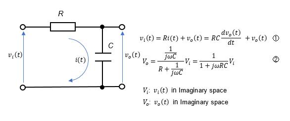
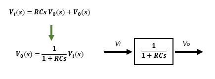
① Model 1 Model of RC filter combining resistor R and capacitor C
When modeling an electric circuit, it is possible to represent it with differential equations, but it is easier to directly create a model in complex number space using impedance expressed in complex numbers, which is familiar in electrical engineering, so I will try to create models in both. In the figure below, (1) is a model of a circuit in real time space using differential equations. In contrast, (2) is a model of a circuit in complex number space.
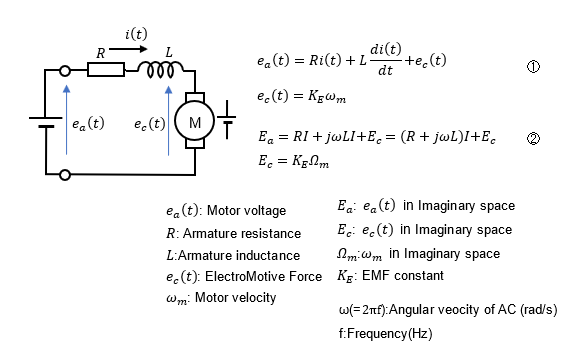
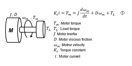
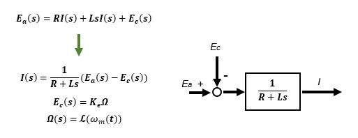
② Model 2 Circuit model of a DC motor (electrical circuit)
The differential equation model of the DC motor electrical system is (1) and the complex space model is (2).
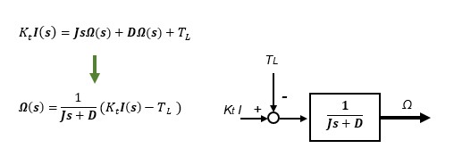
③ Model 3 Mechanical system model of a DC motor (equations of motion)
The first step in modeling a mechanical system is generally to obtain a differential equation model (1) by Newton's equations of motion.
In these examples, a model in real time space with differential equations and a model in complex number space were obtained. In classical control theory, all of these models are analyzed in complex number space, so if the model is a differential equation in real time space, it is transformed using a tool called Laplace transform to represent it as a transfer function in complex number space.
Laplace transform: (transformation from time space to complex number space)
The purpose of Laplace transform in control engineering is to transform differential equations in real time t-space into algebraic equations in complex s-space, which can be easily handled for computation, analysis, and evaluation. The variable s in the Laplace transform is the Laplace operator, which is equivalent to the differential operator, replacing jω with s. After Laplace transform, the mathematical model becomes a block of transfer functions composed of polynomial equations, which can be used to verify input-output and frequency characteristics, and to determine stability.
The Laplace transform itself can be used without understanding the mathematical content, and it is acceptable to separate it as a means of analysis only. If you want to deepen your understanding of the mathematical meaning of the Laplace transform after becoming familiar with it, you may follow the content of the Laplace transform without getting too caught up in the mathematical formulas at first.
After design evaluation of the transfer function transformed into complex space by Laplace transform, the final step is to convert it back to a time function by inverse Laplace transform to check the actual behavior. If the inverse Laplace transform is performed by manual calculation and returned to the time function, it can be evaluated by simulation using Microsoft Excel, etc. However, nowadays, simulation applications can be used to perform the final evaluation without doing any mathematical work.
From a practical standpoint, simulation using manual formulas is convenient and reliable for systems with at most a 2nd-order lag (second-order delay), and for more complex systems, simulation applications are more convenient and reliable. In this case, you don't have to be very conscious of the mathematical part to use it, and the user can concentrate on the essential aspects of the control. In other words, you can design the control with awareness only in the s-space of complex numbers.
As long as you grasp the essence of what you are doing, you can achieve results in the most rational way, regardless of the means.
In the Laplace transform from the time function f(t) to the complex function F(s), f(t) is a function of time t, whereas F(s) after the Laplace transform is a function of the complex number s. In electric circuit modeling(Model1), the differential equation (1) is replaced by a complex function with "s" as the derivative term, and in (2), which has already been created in complex number space, "jω" is replaced by "s", then the result is the same as the Laplace transform, and the both of them match.
There are several Laplace transform formulas, but they are not something you should memorize unless it is for an exam or research. For now, there are a limited number of Laplace transforms that you need to know in order to use them in motion control.
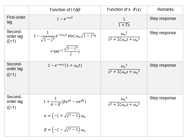
The Laplace transform of differential equations in electrical and mechanical systems can be modeled using 1st- and 2nd-order derivatives and integrals, and the properties of 1st- and 2nd-order lag transfer functions should be understood as the basic forms of transfer functions. 1st and 2nd order refers to the degree of the transfer function denominator polynomial.
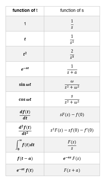
In real-time space simulations, the following formulas are often evaluated using step or ramp signals as input signals, so it is good to know the following formulas.
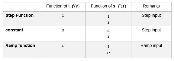
The inverse Laplace transform is used to turn the transfer function G(s) into a real-time space time function g(t) for simulation.
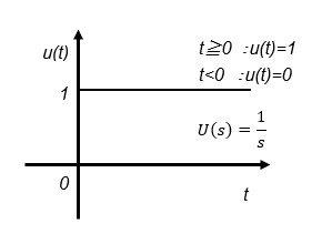
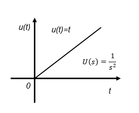
For manual calculation, for example, if the input signal u(t) is a step signal, inverse Laplace transform is performed as G(s)U(s)=G(s)/s, or G(s)/s2 for a ramp function. The step response time functions for 1st-order lag and 2nd-order lag systems are described for manual simulation.
Block Diagram Representation by Transfer Function
The mathematical model created by modeling the control object is converted to a model in complex s-space by Laplace transform to represent the control object as a transfer function in a block diagram. In a block diagram in s-space, the signal transfer from input to output is classified by function like a flowchart and expressed in a visually easy-to-understand manner.
① Model 1 Laplace transform of the model of RC filter
The RC model (1) transfer function between input and output is a 1st-order lag system with time constant RC.
② Model 2 Laplace transform of a circuit model of a DC motor
The DC motor electrical system model (1) expressed by the differential equation is represented by a block diagram with Laplace transform. We can see that the output current I is a 1st-order lag system that returns a back EMF voltage EC when the input is the motor voltage Ea.
③ Model 3 Laplace transform of a DC motor mechanical model
The DC motor-mechanical system model (1) expressed by the differential equation is represented by a block diagram with Laplace transform. The output motor speed Ω is the characteristic of a 1st-order lag system where the input torque KtI is balanced by the load torque TL.
In the previous sections, I have explained modeling, transfer function creation by Laplace transform, and block diagram creation for evaluating and analyzing feedback control in the frequency domain. In the next chapter [Analysis], I will explain how to read block diagrams and the characteristics of first-order and second-order delay systems, which are the basic forms of transfer functions, and then finally explain the intuitive points for designing feedback control systems by combining mathematical formulas and physical perspectives as much as possible.
After designing and evaluating the characteristics in the frequency domain, simulations in the time domain are used to confirm behavior close to the actual one. I recommend an open source simulation application called Scilab. The description can be differential equations such as equations of motion or block diagrams composed of transfer functions, and it is excellent for creating Bode diagrams of not only time response but also frequency response.
Thanks to such a useful tool, it is possible to obtain results without solving difficult differential equations or converting them to time functions based on Laplace transform tables. This has made it possible for us to concentrate on the essence of feedback control, which has lowered the barriers to what is called Control theory and made it a little more accessible.