Fundamentals of Feedback Control using Microcontroller [Analysis]
In "Fundamentals of Feedback Control using Microcontroller [Preparation]" I provide an overview of feedback control and a summary of the process up to the point where the modeled control object is Laplace transformed into complex s-space and a transfer function is created.
In this [Analysis] section, I will explain how to read block diagrams and the characteristics of 1st-order and 2nd-order lag systems, which are the basic forms of transfer functions, and then explain the intuitive points for designing feedback control systems by combining mathematical formulas and physical perspectives as much as possible.
In particular, there are some areas where stability and trackability cannot be explained without using a minimum of mathematical expressions, but the explanations are not difficult and can be understood sensitively.
Table of contents
Transfer function and block diagram (series, parallel, feedback)

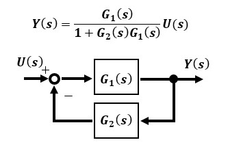
A transfer function is a complex function that expresses the function of converting inputs to a system into outputs. If a system with input u(t) and output y(t) in time space is represented by U(s) and Y(s) in Laplace transformed complex number space, respectively, the transfer function G(s) is expressed as follows.
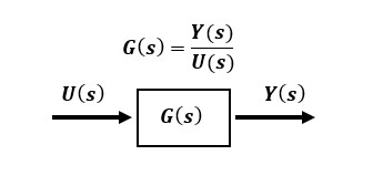
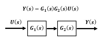
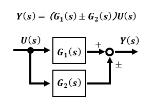
A block diagram is a flowchart-like representation of signal transfer through the transfer function between input and output, classified by function for easy visual understanding. It is sufficient to know the three basic elements.
Transfer function and its characteristics
Especially in motion control, the characteristics of the system can be expressed by a combination of 1st-order and 2nd-order lags, which is the basic form of the transfer function, at a minimum, I would like you to fully understand the characteristics of 1st-order and 2nd-order lags. The other characteristics can be added as needed.
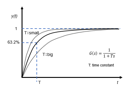
1st-order lag characteristics
When a step input of u(t) = 1 is applied to the 1st-order lag transfer function G(s) at t = 0, the time variation of the output y(t) shows that it is delayed by a certain amount of time (time constant T) relative to the input with an exponential characteristic. Although the output slows with respect to the input, no oscillation occurs. In an electric circuit, an RC filter composed of a resistor R and a capacitor C is called a low-pass filter with a 1st-order lag characteristic, and the time constant T can be adjusted by the parameters of R and C.
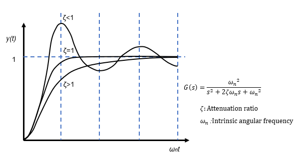
2nd-order lag characteristics
When the 2nd-order lag transfer function G(s) is given a step input of u(t) = 1 at t = 0, the time variation of the output y(t) shows that the response becomes oscillatory or non-oscillatory depending on the damping ratio ζ to the input. The feature of this product is that it can be used in a wide range of applications.
The damping ratio 0 < ζ < 1 becomes oscillatory, and the closer it gets to 0, the greater the oscillation becomes, and at ζ = 0, the system finally becomes a sustained oscillatory system and does not converge.When ζ is greater than 1, the system becomes non-oscillatory, and the larger the value, the harder it is to converge. Empirically, it is said that ζ = 0.6~0.8 is appropriate for servo mechanisms and other tracking control, and ζ = 0.2~0.4 is appropriate for process control and other constant value control. The natural angular frequency ωn is a measure of quick response, and the larger the value, the smaller the vibration period and the better the response.
Physical Considerations
Let me now consider the physical meaning of what is controlled by the 1st-order and 2nd-order lag systems
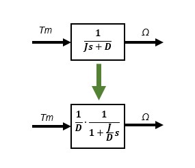
I have modeled a DC motor mechanical system before, so let's take this as an example. If the input is the motor torque Tm and the output is the motor rotation speed Ω, the rotation speed is a 1st-order lag to the motor torque under the condition of viscous friction D.
In other words, when torque is applied to a rotating body, the rotational speed operates with a 1st-order lag. When a constant torque Tm is applied to a stationary free rotating body at a certain point in time (step input), the body begins to rotate from stationary state (speed 0) and keeps rotating at a constant speed when the torque Tm is balanced by the braking force due to viscous friction D.
The physical image of a 1st-order lag system is that it starts up with a delay due to inertia J and viscous friction D in response to this input. The larger the inertia J, the larger the time constant and the slower the startup. As viscous friction D increases, the time constant decreases, but the output rotational speed Ω decreases because the braking force increases.
Next, consider a 2nd-order lag system. Since the rotational position (rotational angle) of a rotating body is the time integral of its velocity, it is a 2nd-order transfer function from the torque Tm, but it is not an oscillating system with a 2nd-order lag because it is just an integral of a stable 1st-order lag system.
Typical of a 2nd-order lag system in dynamics is a model in which a mass m is connected to a wall in the horizontal plane via a spring k and a damper c.
Let x(t) be the displacement when the input f(t) is applied,
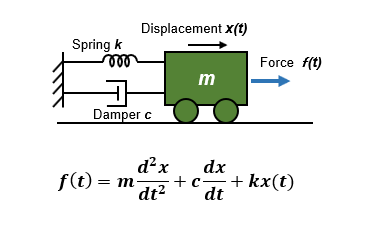
Therefore, Laplace transforming the output displacement becomes a typical 2nd-order lag system with the following transfer function characteristics.
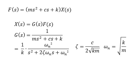
The damping ratio ζ is proportional to the damper c and inversely proportional to the mass m and spring k. As the spring constant k increases, the damping ratio ζ approaches zero, resulting in an oscillating system. As the damper c of the damping element increases, ζ also increases, and the oscillation subsides. The physical image of a 2nd-order lag system is that it starts vibrating slightly in response to the input. If there is no damper c, the system will oscillate continuously without damping.
Transfer function and Bode diagram
In designing mechatronics, including electrical circuits, it is required to be aware of frequency characteristics. A graphical representation of frequency characteristics is called a Bode diagram.
Since the transfer function is a function of the complex number s(=jω) in the frequency domain, a Bode diagram, which is a graph of frequency components on the horizontal axis, is often used as a frequency characteristic between input and output. There are two types of Bode diagrams: the vertical axis is the gain characteristic in gain (dB) and the phase characteristic in phase (°).
What is gain dB? :
Gain dB is the ratio of the Amplitude of the output to the Amplitude of the sinusoidal input in time and space, defined by the following equation
Gain dB = 20log10 Amplitude ratio : Gain Definition
From this, the amplitude ratio in the time-space function is
Amplitude ratio = 10 Gain dB/20
So the Amplitude ratio at 0dB is 1, and the output is the same relative to the input amplitude; the Amplitude ratio is 10 times at 20dB, and , the Amplitude ratio is 0.1 times at -20dB.
What is dec? :
The horizontal axis is also in logarithmic notation in the frequency domain, where "dec" stands for "decade," a unit of measure for logarithmic scale.
This section explains how to view Bode diagrams for 1st-order and 2nd-order lag systems with time constant T.
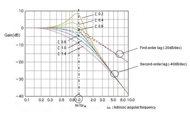
The gain characteristic of the 1st-order lag system has a gain of 0dB up to the natural frequency ωn, which means that the amplitude ratio is 1x and the output is the same as the input, but the gain decreases by -20dB/dec after the natural frequency. In other words, from this frequency, the gain characteristic becomes the same as that of the integral. This boundary frequency is called the cutoff frequency f (=ωn/2π) and is the reciprocal of the time constant T. It has the characteristics of a low-pass filter because it cuts off signals above the cutoff frequency and passes signals only in the low-frequency range.
The gain characteristic of the 2nd-order lag system has a point at which the gain reaches its maximum once at the natural frequency ωn, which is the resonance point of the vibration system. The gain decreases at -40dB/dec after the natural frequency. As the damping ratio ζ increases, the peak gain at the resonance point decreases, and the system becomes a simple low-pass filter. The difference from the 1st-order lag system is that the slope of the gain drop is steeper for the same low-pass filter. This means that it performs better as a filter. The higher the order of the filter's transfer function, the steeper the slope, and thus the better the performance.
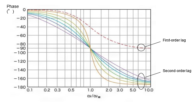
The phase characteristic of a 1st-order lag system shows that it lags behind as the frequency increases, approaching 45° near the natural frequency and 90° at the frequency of infinity.
The phase characteristic of the 2nd-order lag system shows a greater degree of delay than that of the first-order delay system, approaching 90° near the natural frequency and 180° at the frequency of infinity.
Try the convenient tools available on the Internet that will draw a Bode diagram for you when you enter the transfer function parameters and other information.
Transfer function and control system stability
I will now explain the essence of control, which is stability. I will consider the meaning of what is so-called stable and what is unstable from the transfer function equation.
This is not for actually doing a lot of calculations, and although there are some formulas to understand, this is an important part that cannot be avoided in order to understand how a physical phenomenon works in terms of a mathematical equation.
Relationship between the solution (poles and zeros) and stability of the characteristic polynomial
The transfer function G(s), which is generally the s-function between input and output, is expressed as a polynomial in the form
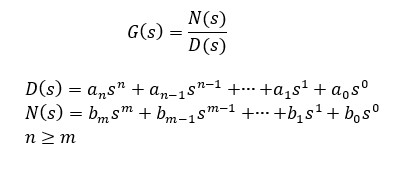
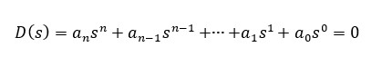
The denominator D(s)=0 is called the characteristic polynomial, and its solution (the characteristic root) is called the pole. In contrast, the solution of the numerator N(s)=0 is called the zero point. A necessary condition for the system to be valid is that the degree of the denominator expression is the same as or greater than the degree of the numerator expression (n≥m).
The stability of a system depends mainly on the position of the poles in the characteristic equation. The word "mainly" means that the zero point also affects the stability of the system, but since this is a bit mathematical to explain and difficult to grasp, I will just summarize the points at the end.
Stability conditions (most important):
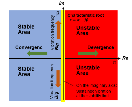
- The system converges and is stable when the poles are all negative real numbers or complex numbers containing negative real numbers.
- When the pole is on the imaginary axis, that is, when the real part = 0, the oscillation is sustained at the stability limit.
- If any one of the poles contains a positive real number, the system diverges.
It is a necessary condition for a system to exist in nature that the order n of the denominator of the transfer function is equal to or greater than the order m of the numerator. m being greater than n means that the transfer function contains a derivative term, but the derivative does not exist in nature because it contains information about the future. Incidentally, the inverse of the derivative, the integral, is the accumulation of the past. To be technical, a system with n≥m is called proper, and a system with n>m is called strictly proper.
Convergence and Divergence
I explain why it is stable when the real part of the poles is negative.
The transfer function G(s) of a system with characteristic equation solutions (characteristic roots/poles) a1, a2, and a3 is expressed by the following equation.

If I do a partial expansion of this and then do an inverse Laplace transform to convert it back to a time function, I get the following.
When t → ∞, the system becomes unstable if even one term in this time function g(t) diverges.
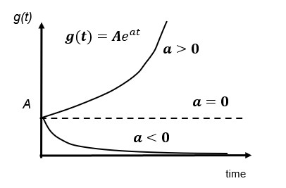
Therefore, the necessary condition for g(t) to be stable over time is that a<0, i.e., that the real number part is negative at all poles. The poles may be complex numbers, and the larger the absolute value of the real part, the faster the convergence, while the presence of an imaginary part results in a damped oscillating system.
If the characteristic root "a" does not contain a real number and is the conjugate root of an imaginary number, it corresponds to the sin or cos function in Laplace transform table 1 in "Fundamentals of Feedback Control using Microcontroller [Preparation]," and thus becomes a sustained oscillation that neither converges nor diverges.
When a=0, the time function g(t) becomes constant, so the transfer function becomes an integrator whose output increases linearly with respect to the constant input.
Up to now, various methods for determining system stability were devised in control theory, but nowadays there are tools for easily solving higher-order characteristic polynomial equations, and characteristic roots can be easily obtained. Even if you don't dare to understand the difficult theory, it can be done to the point, then it's okay to understand only the essence.
Summary of the characteristic roots of the transfer function (solution of the characteristic equation a=α+jβ):
If the imaginary part β of a is 0 (real)
■ Real part of a: α > 0: Divergence
■ Real part of a: α < 0: Convergence
If the imaginary part β of a is not 0 (complex number)
■ Real part of a: α > 0: Divergence
■ Real part of a: α = 0: Sustained oscillation
■ Real part of a: α < 0: Damped oscillation
Output converges with negative real part of characteristic root (the larger the absolute value of the negative number, the faster the convergence), the presence of an imaginary part results in an oscillating system.
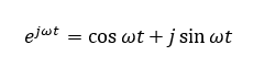
If the characteristic root contains an imaginary number, it will oscillate. This is related to Euler's formula. The proof is a bit mathematical and difficult, but if you are interested, dig in and find out.
About the zero point of the system transfer function
The stability of the system is mainly determined by the position of the poles of the characteristic polynomial, which may not be ignored when zero points are present. In general, the response of a system with a zero point may be worse than that of a system without a zero point, so verification should be performed.
Zeros are not often seen in stand-alone physical elements, but they may appear when coupled with feedback and other factors.
The zero point affects the output according to its positional relationship with the pole. To summarize, the zero point, like the pole, must have a negative real part. If it is positive, it is called an unstable zero point, and it has an adverse effect on the input, such as reverse swing. The closer the zeros are to the poles, the less they affect the input because they cancel each other out. If the zero point is sufficiently far from the pole to the negative side, it will not be affected, but if it is closer to the origin than the pole, it will overshoot, which is not a good thing.
Improved characteristics through feedback
Now that you are familiar with the transfer function and understand the stability of the system, it is time to get down to the business of feedback control. The two main roles of feedback control are as follows.
- To stabilize an unstable control object by applying feedback
- Feedback is applied to improve tracking performance and reduce the effects of external disturbances.
Feedback can stabilize an unstable control object, but the reverse is also true: adding feedback to a stable system may well cause it to become unstable. Therefore, we design a compensator strictly for a system with feedback at the transfer function level, and finally verify the stability and tracking of the entire system.
This concept of feedback applies not only to motion control and other equipment, but also to biology, and we ourselves act unconsciously, but in a very relevant way, on a daily basis. It is interesting to observe the concept as a very deep and philosophical concept, and to apply it to various phenomena.
Stabilizing unstable system
For example, let me trace how a system represented by the following unstable transfer function can be stabilized by adding a feedback loop.
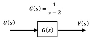
Let me apply feedback to an unstable system with a positive pole in the transfer function G(s) between input and output.
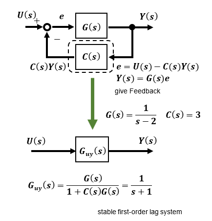
Since the condition for a stable system is that the real-part of the poles of the transfer function is negative, in this case, if I calculate the transfer function Guy(s) between input and output with the compensator C(s) as constant 3, we can see that the original transfer function G(s), which was unstable, has been improved to a stable 1st-order lag system Guy(s) with a negative pole value.
In this way, feedback is applied through the compensator C(s), and the system can be improved by rearranging the system's new pole configuration. The location of the compensator C(s) can be in the feedback loop or just before the control target, but this depends on the control target, so when designing for practical applications, consider the ease of implementation and make a decision based on simulation results.
Internal stability of feedback control

In the previous section, I explained about a simple example of stabilizing an unstable system by applying feedback. In reality, it is not so simple and becomes a bit more complicated when a feedback loop is configured in the system. In a closed-loop system with an additional feedback loop, the closed-loop system must be stable under all inputs other than the target input, such as disturbances and noise added to the system. This indicator is called Internal stability.
The condition for stability is that the output converges without diverging when the target input is given, but it is also important that the output does not diverge when disturbances or noise other than the target value is input.
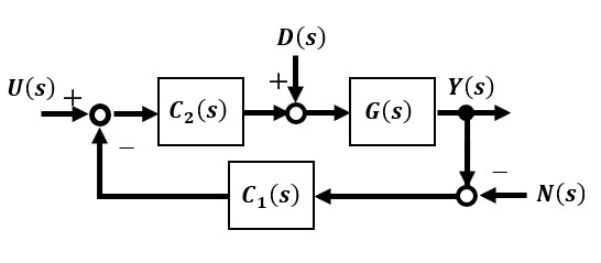
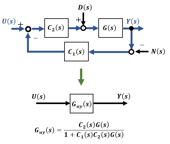
The closed-loop transfer function Guy(s) from the target input U(s) to the output Y(s) without considering disturbances or noise is as follows. First, this closed-loop transfer function Guy(s) must be stable.
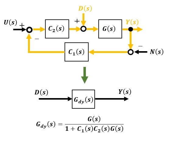
Next, the closed-loop transfer function Gdy(s) from the disturbance D(s) to the output Y(s) without considering the target value and noise is as follows. In the example in the previous section, compensator C2 is 1, so Gry(s) and Gdy(s) are the same. Since the disturbance is generally in the low frequency range, it is preferable to give Gdy(s) the characteristics of a low gain or high-pass filter over the entire frequency range.
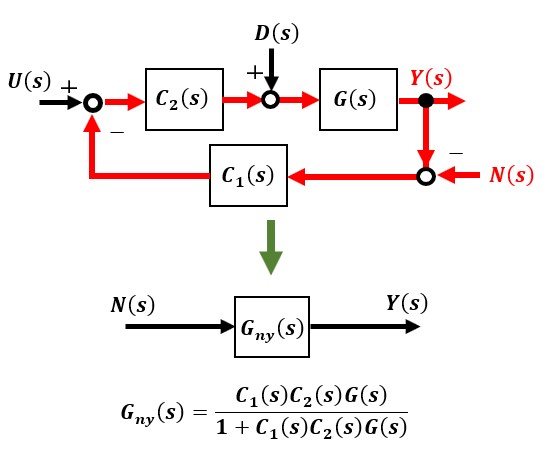
Finally, the closed-loop transfer function Gny(s) from the noise input N(s) to the output Y(s) is as follows. In the example in the previous section, Gny(s)=-3/(s+1), which is stable in this case, but means that the compensator C1(s)=3 amplifies the noise by a gain factor. However, since noise is generally in the high-frequency range, in this example, the noise is passed through Gny(s), which has a low-pass filter characteristic, and does not have much affect on the output.
Disturbance suppression and noise suppression characteristics are often in conflict with each other, and there is a theory that solves this problem called H∞ control, although it is quite mathematically difficult to understand.
There are several methods for determining internal stability, such as the Nyquist's stability discriminant method often found in control engineering textbooks, but in reality, it is often sufficient to determine that the characteristic root of the closed-loop transfer function is stable.
Although internal stability is an important indicator in academia, in motion control using DC motors, the characteristics of originally stable motors are improved, so in my experience, internal stability is not often considered unless a very complicated compensator is added.
Improvement of tracking
Another role of feedback control is trackability. The output to be controlled must follow the target value. Again, this is a conceptual explanation in terms of mathematical formulas, but it is the basis of the concept, so if you understand it well, you will be able to think of physical things in terms of mathematical formulas when you are not sure how to apply the concept in practice.
When you are lost, you will be able to analyze logically, not sensibly, so that you will be able to grasp things from a grounded perspective.
This time, for a more general analysis, I will do so with compensators C1(s) and C2(s) attached to the control target G(s). The transfer function Guy(s) from input U(s) to output Y(s) must be stable.
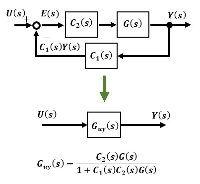
The difference E(s) between the input U(s) and the feedback quantities C1(s)Y(s) is called the deviation, and if the open-loop transfer function G0(s) is assumed from E(s) to the return by loop, the transfer function from input to deviation is as follows.
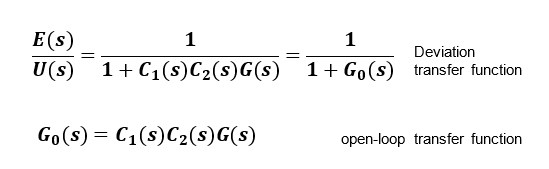
If the time function e(t) of the deviation E(s) converges to a certain value when t→∞ for u(t), the time function of U(s), this value is called the steady-state deviation. The purpose of feedback control is to make this steady-state deviation as stable and close to zero as possible with respect to the input in order to improve tracking performance. For this purpose, compensators C1(s) and C2(s) are designed to be optimal through analysis.
In most cases, actual systems do not have this simple form, but the basic concept is the same for all. In addition to simple step inputs, there are also inputs that vary with time, and following these inputs is called servo tracking.
Let me now verify the steady-state deviation when the system is subjected to step and ramp inputs.
To analyze the steady-state deviation, there is a final value theorem, which is expressed by the following equation.

This is the only thing you may remember.
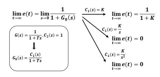
Let me verify the steady-state deviation when a step input and a ramp input are fed back to a stable 1st-order lag system with G(s)=1/(1+Ts), respectively. For simplicity, I set C2(s)=1.
In case step input U(s)=1/s:
When the compensator C1(s) is constant K, a steady-state deviation remains, but when the integrator is set to single-stage K/s or double-stage K/s2, the deviation becomes zero.
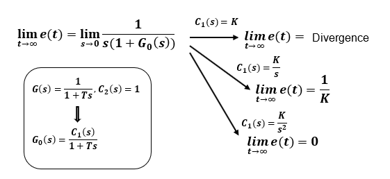
In case ramp input U(s)=1/s2 :
When the compensator C1(s) is a constant K, it diverges, but when K/s with single integrator stage is used, a steady deviation remains but is stable. It can be seen that K/s2 with double integrator stages becomes zero.
The above analysis shows that the steady-state deviation of the system can be reduced to zero by properly setting the feedback compensator, provided that the system is stable.
In a 1st-order lag system, which is stable to some extent to begin with, simply by adding an integrator to the compensator with feedback, it is theoretically possible to eliminate the steady-state deviation so that the output can follow the target value.
In reality, it is not that simple, since there are various disturbances that can cause output to fluctuate, but for a small system, this simple feedback can be very powerful.
There are numerous explanations of control theory in books and on the Internet, but most of them are rather conceptual, like those in university lectures. Those who understand it can understand it to some extent, but even so, it is hard to understand everything because the explanations are mainly based on mathematical formulas, and it is not very interesting. Also, control theory contains a lot of academic content, not just practical, but it is difficult for beginners to distinguish what is really important from what is not.
Therefore, in the "[Preparation]" and "[Analysis]" sections of "Fundamentals of Feedback Control using Microcontroller" only the important parts are excerpted and explained, so that by the time you understand and become familiar with it, the next "[Application]" section will not be too difficult.
In fact, it will be very interesting once you understand the intuition to actually apply what is in the world of theory. In the next issue, I will introduce PID control and other control methods used in the real world, and then use DC motor examples to introduce the intuition for applying feedback control in practice.