Fundamentals of Feedback Control using Microcontroller [Application]

In "Fundamentals of Feedback Control using Microcontroller (Analysis)" I have explained the means to improve the characteristics of a control object by modeling it with mathematical formulas and applying feedback, and to improve the tracking of output to a target value by using mathematical formulas as control theory. From now on, I would like to introduce the application of control theory as a practical technology and confirm how it is actually utilized.
Table of contents
What is PID Control?

PID control is a type of feedback control often heard in the field. PID is an acronym for Proportional, Integral, and Derivative. It may be difficult for those who hear it for the first time to understand what it means, so I will try to explain it.
PID control is expressed in terms of transfer function as follows.
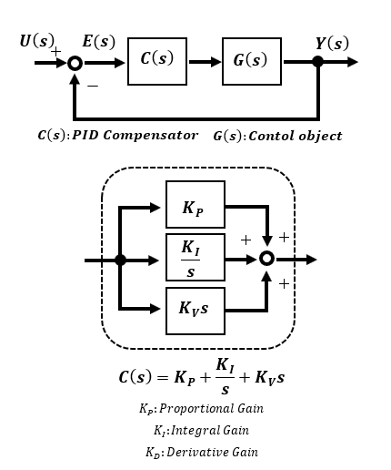
To illustrate this, assume that the control object G(s) is stable with a 1st-order lag. Let u(t), y(t) and e(t) correspond to the time functions of the target U(s), output Y(s) and deviation E(s), respectively.
Proportional P control:
As for the proportional operation, it is easy to understand sensibly: expressed in terms of the s-function, the amount of operation for correction is KPE(s), which is the proportional Gain KP times the deviation E(s). The word "Gain" is used here, but it may be easier to understand if we call it sensitivity. Since the amount of operation is proportional to the deviation (error), it is corrected in the direction that the deviation becomes smaller as time passes.
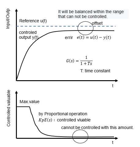
It may seem that this proportional control alone is sufficient, but in reality, due to friction factors in the mechanical system and the control resolution of the electrical system, this deviation is not zero, but is balanced to the extent that it cannot be fully controlled. In other words, it is a characteristic of proportional control that it remains as an offset.
Integral I control:
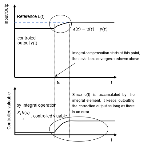
Proportional control inevitably leaves a deviation offset, both in theory and in practice. Therefore, a compensator KI/s with an integrating element is used to converge this deviation to zero. The integrator accumulates the offset portion of the deviation as time passes, so as long as the deviation remains, it continues to correct it to bring the output in line with the target value.
The figure shows what happens when only proportional control is used up to time to and integral control is started after that time. Steady-state deviation remains up to time to, but by including the integral compensator, the deviation accumulates and continues to be corrected, bringing the steady-state deviation that cannot be handled by proportional control close to zero. However, if the control target is a 1st-order lag system, the integral compensator will cause a 2nd-order lag system, which may lead to instability depending on the gain selection.
Derivative D control:
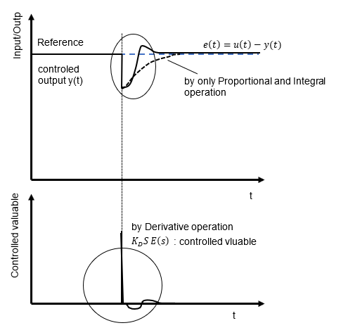
Finally, there is the correction by the derivative compensator. Derivative compensator works when there is a time variation in deviation. For example, if the output changes abruptly due to a disturbance, it is corrected according to the change. The purpose is to converge the deviation as quickly as possible in response to sudden changes.
The derivative compensator has the opposite characteristics of the integral compensator, and since future information on derivative action cannot be obtained in reality, it is realized by approximate differentiation. Since it also has the property of advancing the phase, it also serves to compensate for phase deviations caused by first-order delays and the like.
Due to its nature, the differential compensator is good for temperature regulators and other relatively slow control objects, but care must be taken when using it in motor control, electric circuits, and other fast-response systems, because if used incorrectly, it can act too sensitively and become unstable. It is effective when used for applications that require rapid correction.
Feed-Forward Control
Feedforward control is relative to feedback control, but whereas the input for feedback control is only the deviation between the target value and the feedback value, the feedforward input provides information other than deviation, such as the target value.
A relatively stable system can function with only feedforward input through so-called open-loop control, but a feedback control system is used to improve the accuracy of the output or to make the system more resistant to disturbances.
Adding feedforward information to the input of such a system may make the system more stable because it does not have to rely solely on feedback information.
In designing a system, it is up to each person to decide whether to view it as a feedforward compensation mainly based on feedback control or feedback compensation mainly based on open-loop feedforward control.
There is a concept of disturbance observer, which estimates uncertainties due to disturbances and system fluctuations in what is called robust control, and provides the feedback-driven system with information to cancel the estimated disturbance as feedforward compensation.
Speed control of DC motor
There are many different types of electric motors, but DC motors are the ones most often covered in control theory. This is because DC motors are easy to model electrically and mechanically, and they are controllable simply by changing the DC voltage to the terminals without the need for a dedicated drive device. Also, the characteristic that the torque generated by a DC motor is proportional to the armature current makes it easy to apply as an actuator in a control mechanism.
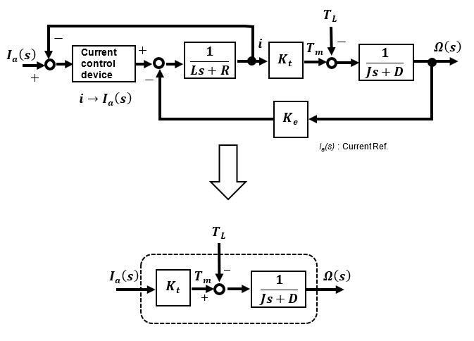
Let's start by creating a block diagram using the transfer function model derived from the electrical circuit and equations of motion of a DC motor to check its characteristics. The block diagram of the electrical and mechanical systems of a DC motor derived in [Preparation] can be summarized as follows.
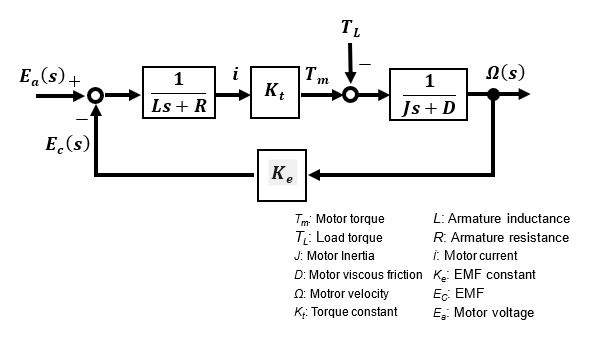
From the block diagram, if the input of the DC motor is the motor terminal voltage Ea(s) and the output is the motor rotation speed Ω(s), its transfer function is a 2nd-order lag system due to the inductance L of the electrical system and the motor moment of inertia J of the mechanical system.
In fact, when voltage is applied to a DC motor, the rotational speed is relatively stable and not oscillatory. This is because the effect of the inductance component of the motor is much smaller than the effect of the moment of inertia of the mechanical system, resulting in almost 1st-order lag system characteristics. Therefore, if the inductance is set to L=0 and the viscous friction D of the motor mechanical system is also set to D=0 for simplicity, an approximate model is created as follows.
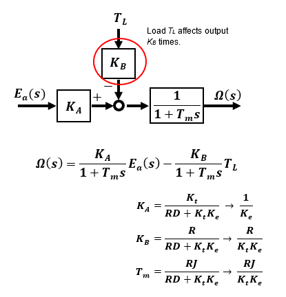
Without load TL=0:
The output rotation speed Ω(s) with respect to the input Ea(s) is a 1st-order lag with time constant Tm. In no-load operation with load torque TL=0, the output rotational speed is proportional to the input voltage with a 1st-order lag. This is why DC motors are easy to handle in so-called open control, where the rotational speed can be changed simply by changing the applied voltage.
With load TL≠0:
When a load TL is added, KB times the TL will affect the rotational speed output. In other words, the rotational speed cannot be adjusted to any desired speed in a method that only changes the applied voltage of a DC motor by open control, because the rotational speed is affected by the load. The response is determined by the parameters of the motor's electrical and mechanical systems, which is the limitation of the performance of open control speed control of DC motors.
In this article, I would like to check the characteristics of a system that uses a PI control compensator to maintain Motor speed through speed feedback. The block diagram is shown in the figure below.
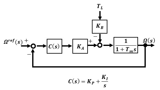
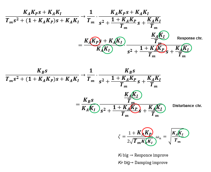
The response characteristics from the reference(target) value Ωref(s) to the output Ω(s) and the disturbance characteristics from the disturbance TL to the output Ω(s) are integrated in the compensator to form a 2nd-order lag system.
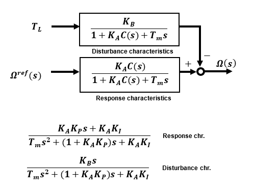
Proportional P control
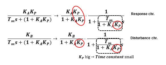
First, let's look at the characteristics when only the proportional compensator functions (KI=0). Both response and disturbance characteristics become a 1st-order lag system, and adjusting the proportional gain Kp reduces the time constant and improves response. As for the disturbance characteristics, if the proportional gain Kp is sufficiently large, the effect is reduced. However, the steady-state deviation, which is a characteristic of the 1st-order lag, remains.
Proportional-Integral PI control
So, let's look at the characteristics when an integral compensator is added. The damping ratio ζ can be set mainly by the proportional gain KP and the natural frequency ωn by the integral gain KI. The effect of disturbance characteristics can be reduced if the integral gain KI is sufficiently large.
However, the selection of these gains Kp and KI is not an easy task, and in some cases, such as the attenuation ratio in this case, they may interfere with each other, so a certain amount of trial and error is required.
Current-controlled drive of DC motor
Until now, the operation to control a DC motor has been based on the input of the applied voltage Ea(s) to the terminals. This is because DC motors can basically be operated at variable speeds even in open control by operating the applied voltage. In actual operation of a DC motor, variable speed operation can be easily achieved by directly supplying a PWM pulse signal with a duty ratio proportional to the voltage as a driver input using a voltage control type driver.
Why use DC motor with current control?
In the previous chapter, it was confirmed that the characteristics of the system can be improved when feedback control is applied to make speed operation more stable. However, while the voltage control type, which operates the applied voltage of the motor, is convenient for small variable speed applications, its performance improvement is limited for more precise control of rotational speed, angle, and torque in industrial applications.
This is because DC motors are affected by back EMF and the motor electrical system, as can be seen in the block diagram model of a DC motor. The current control type, which directly operates the motor current, is not affected by the electrical system because of its linear characteristic where the armature current of the DC motor is proportional to the drive torque, and can directly operate the part close to the mechanical system. In addition, the voltage input type is susceptible to input limitation by the voltage upper limit, making it difficult to demonstrate its performance. For these reasons, many control operations as actuators for more serious motion control are performed with current.
Driving a motor by current operation is easiest with a current-controlled type driver, but other methods include a hardware or software feedback control system that detects the motor current and configures a feedback control system as a current loop. Current control depends on the driver, but generally, an analog voltage is used as the current command value, and MCU with a DA conversion function is used.
DC Motor Driver
TB6612FNG is a driver module that can connect up to two DC motors and is a voltage control driver module that gives voltage commands in PWM pulses.

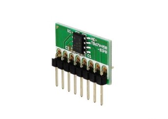
TB67H450 is a driver module that connects one DC motor and can perform voltage control by giving voltage commands of PWM pulses like TB6612FNG and current control by giving analog voltage as current commands.
What is called advanced control (robust control, 2-degree of freedom control)
Advanced control is a control method that is an extension of classical control and modern control theory, and has strong robustness against fluctuations caused by external disturbances and errors due to modeling uncertainty.
I have described the design evaluation process from modeling the control object into a mathematical equation, but in practice,
1.Model parameter uncertainty
2.Adverse effects of disturbances, noise, etc.
3.Variation of characteristics due to load, operating conditions, etc.
It is almost impossible to model perfectly due to such factors. Robust control is control that does not degrade control characteristics, including stability, even when the target to be controlled is subject to uncertainty or variation as described above.
In PID control, no matter how much you try to improve the tracking and disturbance suppression characteristics, they interfere with each other, so no matter how optimally you select the gains, you will not be able to achieve characteristics that satisfy both.
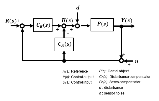
In contrast, 2-degree of freedom control is one of the robust control types. This control system allows independent design evaluation of the so-called disturbance suppression characteristics against modeling uncertainties and fluctuations and the tracking characteristics, which is the original purpose of control, so that both characteristics can be optimized.
The compensator CA(s) improves the robustness against fluctuations due to disturbance d and noise n, and the compensator CB(s) improves the trackability of the output Y(s) with respect to the target value R(s), which are called 2-degrees of freedom because CA(s) and CB(s) can be set independently of each other.
The methods for improving robustness are profound and this is a very advanced level of control theory, so I will only introduce it here. I would like to try again and summarize when I can actually do a little verification not only with theory but also with microcontroller applications. Please refer to the next chapter "Fundamentals of Feedback Control using Microcontroller [Advanced]" for details.
I have summarized the contents you need to understand in order to realize a motion control application using MCU in the following sections: [Preparation], [Analysis], and [Application] in a lecture style. This is not simply a summary of the contents of textbooks, but rather a bible note of excerpts that are necessary based on the actual results of motion control cultivated through practice, so it should be very useful in practice for beginners who are just starting out in the real world of control.
Feedback control should be used based on a solid theory, not just a set of parameters based on a feeling when designing and using it in practice.
Please look forward to the "Applications and practices" section, where I plan to explain specific methods for various applications using DC motors as motion control.