Fundamentals of Feedback Control using Microcontroller [Advanced]

In "Fundamentals of Feedback Control using Microcontroller [Application]" I explained PID control, which is used in practice based on classical control theory. PID control is easy to use in the field when the model to be controlled is relatively simple, because the gain can be set sensibly. However, when the influence of parts that could not be modeled due to external disturbances or parameter fluctuations of the controlled object is large, the desired performance cannot be expected.
Therefore, this part introduces what is called Advanced control, which uses a DC motor as the control model and is a development of conventional classical control theory. The objective is to achieve the expected performance even in the presence of disturbances such as modeling errors and load fluctuations, which are unavoidable in practical applications.
Speaking of advanced control, there are many typical examples such as robust control and adaptive control, but they are considered to be academic and unrelated to general applications because of their high level of difficulty and theory-centered explanations.
Here I will introduce something that can be used immediately in practice and explain something practical that anyone can use.
Table of contents
- 1 Robust control resistant to model errors and disturbances
- 2 2-degree of freedom control system
- 3 Approximate models handled by robust control
- 4 Stable speed control in the presence of modeling errors and disturbances
- 5 Comparison with High-gain feedback method
- 6 Positioning tracking control (Acceleration command method)
Robust control resistant to model errors and disturbances

Among the advanced controls, robust control will be explained in this article.
Robust control refers to a control system in which the control output is not easily affected by disturbances on the input side of the control target P(s), such as modeling errors and load fluctuations when a physical control model such as a DC motor is converted into a mathematical expression, and disturbances on the output side of the control target, such as sensor noise.
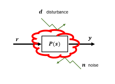
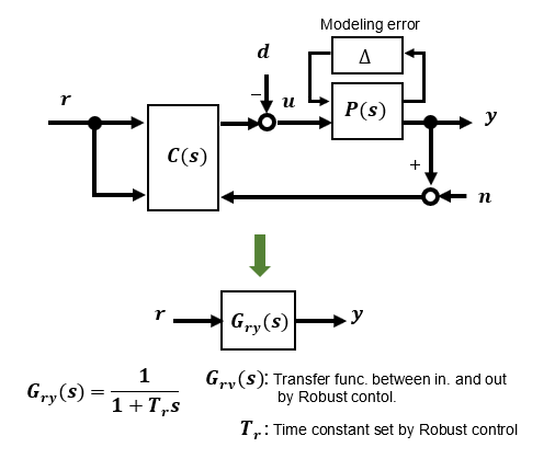
In robust control, the compensator C(s) is designed so that the transfer function Gry(s) from input r to output y has a set characteristic (e.g., 1st-order lag with time constant Tr) even in the presence of disturbance d, observation noise n, and some model error ⊿.
Among robust control methods, if it is as simple as PID control, I would like to actively apply it to small applications. In this part, I would like to verify such practical applications that can be handled with relative ease.
2-degree of freedom control system
Conventional PID control adjusts the output by setting the proportional, integral, and derivative gains of the PID compensator in the feedback loop, respectively. Each gain is often determined by trial and error, with values based on experience.
The advantage of PID control is that it can be set easily and sensibly without theoretical understanding, but the gain can only adjust the response, not fundamentally improve the characteristics against external disturbances.
In addition, conventional feedback control such as PID control can improve stability and response by increasing the gain in the loop (amplification), but at the same time, it can also amplify modeling errors, noise, and other unwanted effects, which may result in failure to achieve the expected performance. The There is a limit to how much improvement in accuracy and responsiveness can be hoped for with mere feedback control.
To achieve robust control, there is a control method called a 2-degree of freedom control system in which the response characteristics and disturbance suppression can be set independently. There are other robust control methods, such as a disturbance observer method that estimates disturbances and modeling errors and cancels the changes, but this part deals with 2-degree of freedom control.
There are various types of 2-degree of freedom control, but the one I will be dealing with here is the simplest, easiest to verify by anyone, and the easiest to realize through programming.
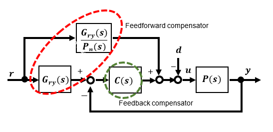
The block diagram from input r to output y takes the form of the figure below. In addition to the usual feedback control loop, information branched from the input is added.
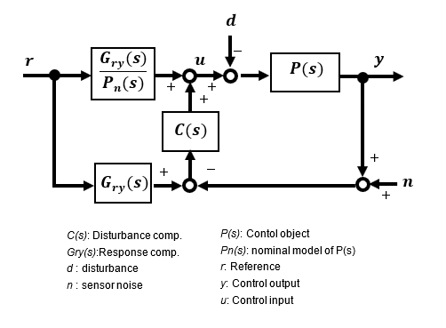
Rearranging the block diagram above yields the equivalent block diagram shown below. What this means is that it consists of a feedback section and a feedforward section. Disturbance suppression is improved by the feedback compensator C(s), and response characteristics are improved by Gry(s) and Pn(s) in the feedforward section. Since these can be set independently without interference, they are called 2-degree of freedom.
Approximate models handled by robust control
In "Fundamentals of Feedback Control using Microcontroller [Application]", I explained that the motor rotation speed can be adjusted by changing the input voltage. Since the rotation speed is almost proportional to the input voltage when there is no load, the motor can be approximated by a 1st-order lag as shown in the figure below, where u is the input and y is the output.
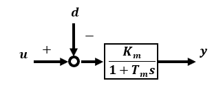
The approximate model gain Km and time constant Tm are obtained by actually measuring the rotational speed y when given the actual input. This is called a kind of parameter identification, but these are approximate model parameters rather than physical parameters such as the actual moment of inertia J or viscous friction D of the DC motor.
This model is more practical because the physical parameters from input u to output y are concentrated in Km and Tm. The input can be either a voltage or a current, and the parameters Km and Tm are correspondingly valued. Km is the gain of the transfer function, but it may be easier to understand as a conversion factor from input to output.
Depending on the control application, it is not very meaningful or practical to go into too much detail in search of accuracy when formulating a physical model. Parameters fluctuate, and disturbances are always present. Since control is based on a mathematical model, a model with minimum characteristics is necessary, but for robust control, a simplified model of the control target is acceptable, especially in the case of robust control.
Stable speed control in the presence of modeling errors and disturbances
Speed control using a 2-degree of freedom control system with a DC motor as the control target will be explained.
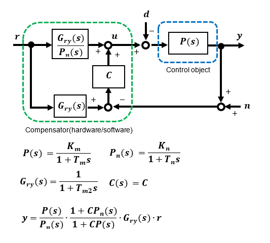
The control object P(s) is a 1st-order lag model with input u as voltage or current and output y as motor rotation speed. This real model has parameters Km and Tm that may vary, but let Pn(s) be this nominal model.
The parameters of the nominal model Pn(s) are the parameters Km and Tm obtained from the parameter identification of the real model P(s) as the normative model parameters Kn and Tn, respectively, which are used in the feedforward compensator.
The feedforward compensation section consists of the reference response characteristic Gry(s) between input and output after characteristic improvement and the inverse system Pn (s) -1 of the nominal model, and the feedback compensation section contains the gain C (constant this time depending on the control target) that determines the robust characteristic.
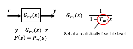
The reference response characteristic Gry(s) between input and output after characteristic improvement is assumed to be the 1st-order lag of the time constant Tm2, but the time constant Tm2 must be set at a level that can be realized.
Response characteristics without modeling error in the control object P(s):
If there are no error variations in the real model P(s) and the nominal model Pn(s) under control and P(s) = Pn(s), the transfer function from input r to output y is the set reference response characteristic Gry(s).
Response characteristics with modeling error in the control object P(s):
If there are error variations in the real model P(s) and the nominal model Pn(s) to be controlled, ⊿(s) in the figure below represents the variation. The larger the feedback gain C, the smaller the effect of the fluctuation error, and thus the closer to the set reference response characteristic Gry(s).
Another feature of the type of feed-forward compensation set up in this case is that the real and nominal model parameters cancel each other out even when there are fluctuations.
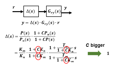
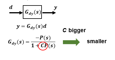
Affect of disturbance on output:
This is the essential part of 2-degree of freedom robust control. The disturbance characteristic is related only to the feedback gain C and is independent of the reference response characteristic Gry(s), which determines the response characteristic.
It can be seen that the larger the gain C, the smaller the effect on the output. This value should also be set within a feasible range.
If you want to eliminate the Steady state deviation:
In this 2-degree of freedom control, the reference response characteristic Gry(s) is a 1st-order lag, so if the load torque is constant and large, as in a steady-state load, a steady-state error will occur. To reduce this error, increasing the feedback gain C will bring it closer to zero, but it will not converge completely.
Inevitably, to make the output match the target value completely, a PI feedback compensation loop is added to eliminate the steady-state deviation on the outside and adjust the appropriate proportional and integral gains.
The key to implementation is to process the robust control section as fast as possible, and process the servo compensation loop with PI feedback slower than that to eliminate the effects of mutual interference.
In the case of speed control, the robust compensation gain C makes the effect of disturbances almost negligible, so there may not be much point in adding a PI control loop to eliminate steady-state deviation unless the application is to maintain a constant speed with high accuracy regardless of the load.
Verification by simulation (2-degree of freedom robust control)
Output response in DC motor open loop condition:
The time response of the verified results is verified by simulation (using Scilab).
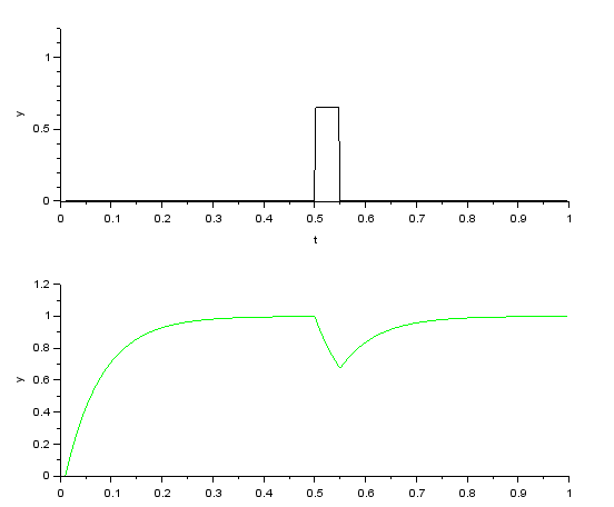
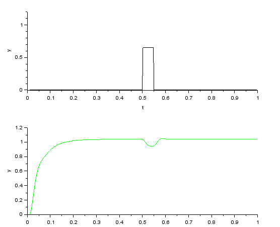
This is the response when a DC motor is subjected to a pulse-like load disturbance at the step input in open-loop condition. It can be seen that even a small pulse-like load has a large effect on the output.
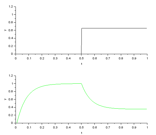
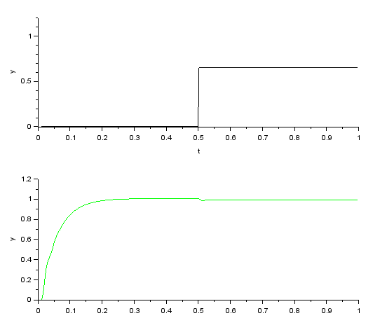
This is the response when a step-like load disturbance is applied. The torque is balanced with the torque generated by the load at the point where the load has dropped significantly from the command value.
2-degree of freedom robust control Output response:
This is the output response of the target response characteristic Gry(s) when a pulse-like disturbance is applied under the conditions that the time constant Tm2 is 50ms and the robust compensator gain C is 0.5. In addition to model errors of +30% for Km and -20% for Tm with respect to the nominal model, a 1st-order lag parasitic element with a time constant of 10ms is added to the control object, resulting in a 2nd-order lag system. The result is a very good example of this.
Further increasing the robust compensator gain C improves the suppression of fluctuations in disturbances and modeling errors.
This is the response when the disturbance is step-loaded after increasing only the robust compensator gain C to 3. Again, the output maintains the target response characteristic Gry(s), and the effect of the robust control can be seen as the effect of the disturbance is almost nonexistent on the output. This is a good example of the effect of 2-degree of freedom control, which allows the response characteristic and disturbance suppression characteristic to be set independently.
Comparison with High-gain feedback method
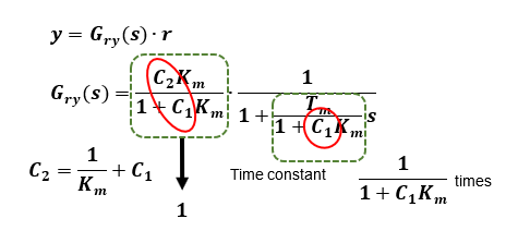
A simple method to improve speed control characteristics is the High-gain feedback method. This is a very simple method in which the output side is fed back through gain C1, and the gain between input and output can be brought close to 1 while suppressing disturbances by combining the values of gains C1 and C2.
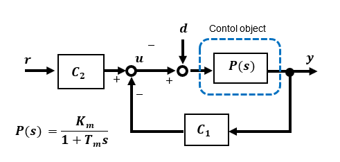
To improve the disturbance characteristics, the disturbance suppression feedback gain C1 can be increased, which is called High-gain feedback because it relies on the magnitude of C1.
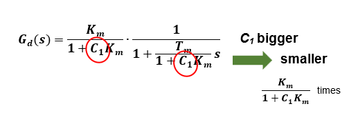
The response characteristic can be obtained by adjusting C2 so that the overall gain becomes 1, but it depends on the size of the disturbance suppression gain C1 and cannot be obtained arbitrary response characteristics. In addition, since it relies on high gain for disturbance suppression, care must be taken to ensure that it is not affected by noise from the output-side sensor.
High-gain feedback is useful for applications that do not require robust control and where the effects of disturbances are relatively small. It is advisable to use the two different types of feedback depending on the application.
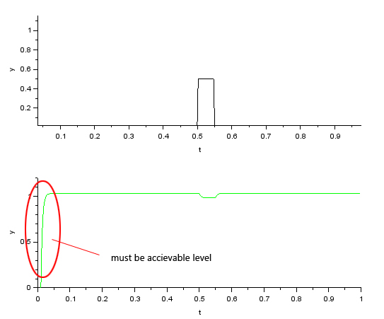
Verification by simulation (High-gain feedback)
Simulation results of the response to a pulsed disturbance load. The disturbance pulse is suppressed by feedback gain C1, but at the same time the response is affected, resulting in over-response depending on the gain and modeling parameters.
Disturbance suppression and response characteristics are determined by the feedback gain C1, but the High-gain feedback method is the simplest and most practical if it can be set within a feasible range.
Positioning tracking control (Acceleration command method)
If the speed control model is modeled with a reference response characteristic Gry(s) that is not affected by disturbances or modeling errors, it can easily be developed into a positioning tracking control. This section describes the Acceleration command type positioning tracking control, which is different from the type that consists of a position control feedback loop outside of a velocity control feedback loop, which is often seen in industrial applications.

The time constant Tm2 of response Gry(s) should be set small enough to be feasible.
In order to generate acceleration command values, the target values of the following trajectory for position θ0, velocity θ'0, and acceleration θ"0 are created in advance. The acceleration command value θ"ref is consist of the acceleration reference value θ"0 used as the feedforward term, and the error between the velocity θ'0 and the position θ0 reference value and the actual values θ and θ' multiplied by the gains Kv and Kp, respectively, as feedback terms.
The gains Kv and Kp can be easily determined with reference to the response of the 2nd-order lag system, taking into account the quick response and damping of the target. When the error at startup is converged by the response of the set 2nd-order lag system, Δθ(=θ0 -θ) is 0, which means that the actual position θ follows the reference value θ0 without delay.
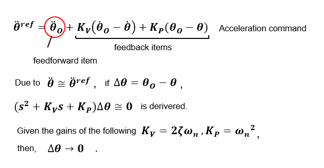
The above equation is valid because robust control is applied to the velocity system and the velocity command value θ'ref ≈ velocity θ', which means that the acceleration command value θ"ref ≈ acceleration θ".
Looking at the above equation, it seems that the gains KV and KP can be determined arbitrarily, but if the gains are selected appropriately, the response may be disturbed. This is because these gains are used to construct a 2nd-order lag system normative model.
When viewed as a position command system, if only the target value θo is given as the command value, the transfer function from the target value θo to the output θ is KP/(s2+KVs+KP), the normative model of the 2nd-order lag system, and the output θ follows with a delay.
By including acceleration θ"ref and velocity θ'ref in the command values for the normative model, they play a feed-forward role in the position command system, eliminating steady-state deviation and allowing the system to follow without delay.
In other words, the normative model must be stable as a system, and if we construct an inverse system of a normative model with unstable zeros to a normative model with unstable poles, there seems to be no problem since they cancel each other out in the equation, but in reality, there are always lag factors, modeling errors, disturbances, etc., so they do not cancel each other out and remain unstable.
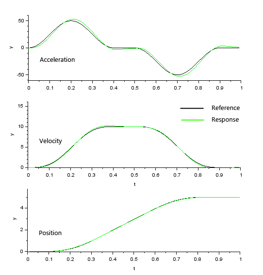
Verification by simulation (positioning tracking control)
I simulated the tracking performance of the reference response characteristic Gry(s) when the time constant Tm2 is 10ms and the gains Kv and Kp are Kv=16 and Kp=100, assuming quick response ωn=10 and damping 0.8. The simulation results show that the position can be tracked even if the time constant is large, since the command value is relatively slow.
Robust control is an advanced category of control and may have been unrelated to general or hobbyist applications, but the control methods introduced here can be easily applied to motor control using a small MCU program.
Usually, in the case of voltage input DC motor control, even if feedback control is performed from an encoder, etc., if PID control is used, there is not much hope of improving the characteristics, but if the 2-degree of freedom robust control and High-gain feedback described in this article are applied, the effects of external disturbances can be suppressed, so it can be used as if it were a stepper motor. This allows the motor to be handled, which broadens its application.
Verification by simulation is performed under unrestricted input conditions. In the case of implementation, motor terminal voltage and maximum current will be restricted, so it is necessary to check whether it is feasible or not by including the conditions of the physical model. In the next issue, I would like to conduct verification using an actual device.