Physical interpretation of impulse response and its transfer function

I have tried to verify how the function g(t) in the time domain between system inputs and outputs has characteristics depending on the input signal. For this verification, we need an impulse response, so let's start with the main points about an impulse signal. Impulse response is not something we are usually aware of when dealing with mechanical motion control, but it is something we often see in control theory. It is often used in signal analysis of electrical systems.
In transfer function notation in s-space, the input U(s), the control object G(s), and the output Y(s) can be interpreted separately, but the characteristics of the time domain function g(t) are a composite of the input signal u(t) (that is, y(t)=g(t)), making it difficult to grasp the reality.
Therefore, I will verify the characteristics during the impulse response, comparing it to the response when a step input is given to the system, and discuss what it means in terms of mathematical interpretation and physical phenomena.
Table of contents
Definition of impulse input

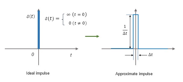
An impulse input is one whose time width is infinitesimal, whose amplitude is infinite, and whose integral is 1. Although not feasible, it is useful for examining system characteristics on a mathematical equation.
When an instantaneous and shocking impulse input is given to a system, the response of the system itself shows it's characteristics whether it is stable and converges or unstable and diverges. This is the impulse response.
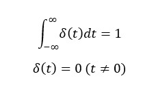
An ideal impulse signal cannot be generated in reality, so an approximation should be used for testing, etc.
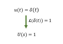
The impulse signal is also characterized by the fact that it is 1 when Laplace transformed. This means that when inverse Laplace transforming the impulse response characteristics of the system transfer function to the time domain, we are examining the characteristics of the transfer function itself, since the input in the s-domain is 1. This is an important part of the impulse response.
Response by Input
Now that I know what an impulse input is, we will compare it with a step input to the system.
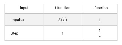
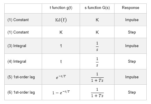
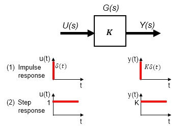
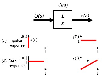
The table below shows the time function g(t) when the system transfer function G(s) is given an impulse input and a step input, respectively, with constant K, integral 1/s and 1st-order lag 1/(1+Ts).
Below is a graphical interpretation of what the output will be for an input when the system is constant, integral, and first-order delayed.
If the transfer function in the s-domain is constant (1) and (2), the system in the time domain can also be understood as sensible. For example, if the transfer function is a constant K, the output will be K times K for an input of 1. Even in the time domain, the output will be K for an input of 1. Under all conditions, the output is K times the input.
Next is the case (3) and (4) where the transfer function is integral. From the mathematical interpretation of the meaning of integration and the definition of an impulse signal, it is clear that the response to an impulse input is a fixed value of 1, while the integral response to a step input is a linear increase in output. When interpreted from the transfer function in the s-domain, there should be no hesitation in understanding it in this way.
Now let us consider the opposite case, starting from (2) and (3), where the time domain system is 1 or constant. That is, when g(t) = 1 (constant). What does this mean physically? It is a bit difficult to interpret, but it means that there is no change in the output relative to the input, i.e., no change in the state of the system over time.
Since this is a bit abstract, a concrete example will be explained using the equations of motion in the next section, "Interpretation in Equations of Motion".
However, when analyzing the characteristics of the system itself, we will only deal with (3) because it is a case of impulse response.
Finally, there are cases (5) and (6) where the system has 1st-order lag characteristics. It is easier to interpret the behavior intuitively compared to the integral characteristic.

Interpretation in Equations of motion
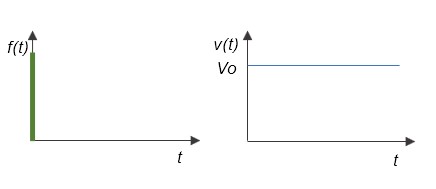
To interpret the integral property physically, consider the velocity v(t) of an object of mass M, neglecting friction, subjected to an external force f(t).
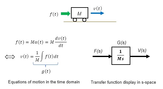
In the equation of motion in the time domain, the acceleration a(t) produced by the external force f(t) is proportional to the mass M. In other words, if the input is the external force f(t) and the output is the acceleration a(t), the transfer function between input and output corresponds to the constants (1) and (2).
Since the velocity v(t) of an object is the time integral of the acceleration a(t), v(t), in terms of the external force f(t), is through the integrator.
This is where we come to the main issue. When an impulse input is applied to a stationary object as an external force, it begins motion with an initial velocity VO and continues constant velocity motion with VO due to inertia caused by mass M in a frictionless space (3). In other words, there is no change in the velocity state v(t) with respect to the input over time.
This is the physical interpretation of an integral operation in which the time function g(t) of the system is constant.
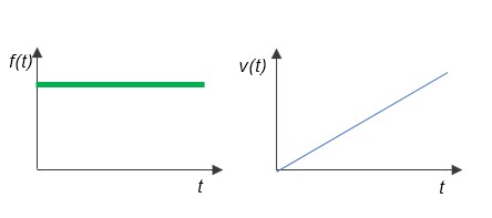
If the external force f(t) is a step input, the object is in equi-accelerating motion with constant acceleration a(t), and the velocity v(t) is an integral motion (4) that increases linearly.
Since the Laplace transform of the step input itself is 1/s, the same as the integral, the output will be a ramp function with the 1/s2 property when the step input is given to the integral system.
The horizontal projection often seen in high school physics textbooks and reference books is a constant velocity linear motion with initial velocity Vo due to impulse input, while the vertical direction is a constant acceleration motion with acceleration "g" due to gravity, equivalent to a step input in free fall.
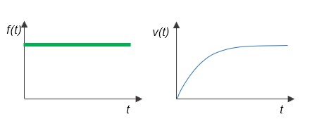
Since friction exists in reality, if an external force f(t) is given as a step input, it will balance the frictional force and the velocity v(t) will have a 1st-order lag.
Postscript:
The impulse response is useful for verifying the response characteristics of the system itself, and was explained in comparison to the practical step response. Even what we take for granted as formulas in mathematical expressions may not be explained well without a complete understanding. The combination of impulse, step response, and integration, which was the focus of this lecture, was also surprisingly difficult to understand completely. If there are other examples like this, I will try to interpret them with a legend as much as possible.